Maps are used in software applications all the time - from routing when driving, to ordering takeout, to finding new parks in town. These applications provide users the ability to search for geographic points of interest in a specific geospatial area. To support mapping functionality in a performant manner, understanding approaches to optimally store this geospatial data is critical. In this article we cover seven approaches to storing geospatial data.
Terminology:
- Geocoding - converting address to geocoordinates
- Geohashing - converting two-dimensional geocoordinates to a indexable string
- Hilbert Curve - a mapping between 1D and 2D space that preserves locality
2D Search
The first and simplest approach we call 2D-Search. With 2D-Search we store the data in a generic relational database and scan the whole table with a SQL query condition for lat in range and long in range. As you can imagine, this is highly inefficient as we are scanning through every row in the table. Even if we were to index by latitude and longitude individually we will end up querying the intersection of two massive datasets (eg. get all points with lat in range, get all points with long in range, filter). This type of indexing only improves lookups in one dimension so we still end up filtering through the second dimension. The fix for this is some form of spatial hash indexing.
Even-Grid Hashing
A very basic form of spatial indexing is the simple Even-Grid Hashing approach. In an Even-Grid approach, we improve on the basic SQL table scan by hashing the latitude and longitude of each point into a string and dividing the map into a grid of fixed equal areas. When a query is submitted, the coordinates are hashed to look up the cell containing the target and then points within that same cell for results. This is an improvement over 2D-Search as we are only looking at the dataset of the current cell, but it is fatally flawed in two ways. First, by using cells of only a single fixed size we need to filter large numbers of results, especially near borders, and inversely in sparsely-populated areas there may not be enough results. Some areas of a map, such as in cities, will have far more points of interest than others creating hotkeys. Second, by not searching adjacent cells for points nearby, we will miss important points of interest which are nearby but just beyond a cell border. The fix for this is Geohashing.
Geohashing
The third approach and first realistic option for us to consider is Geohashing. In 2008, Gustavo Niemeyer published his work publicly on Geohashing and its adoption has since become wide-spread in geospatial applications. Geohashing divides the map recursively into smaller grids of cells with each additional bit, providing multiple resolutions of cells dependent on query hash length. Queries first have their latitude and longitude hashed into a string, similar to the previous approach, but then multiple cells are queried at various resolutions. For example, an area fully within the radius of a search could use a larger resolution cell, whereas areas near the maximum radius of a search could use smaller resolution cells covered proportionally by the search. Dividing the map recursively, the first iteration divides the map into 4 quadrants: 01 for the NW quadrant, 11 for the NE quadrant, 00 for the SW quadrant, and 10 for the SE quadrant. On the second iteration each of these quadrants is further divided; for example 01 becomes 0101 for NWNW, 0111 for NWNE, 0100 for NWSW, and 0110 for NWSE. This continues recursively to the desired granularity, up to 12 bits. With the largest granularity, 1 char, each cell covers 1,600 miles, whereas with the smallest granularity, 12 chars, each cell covers a couple inches. For our use-case we will support 4 chars (~12mi radius) up to 6 chars (~1/4mi radius).
Geohashing guarantees the longer a shared prefix two points share the closer they are located to each other. The primary issue with geohashing is the inverse is not guaranteed - two adjacent cells in a grid near grid-division boundaries may not share a common prefix at all even when right next to one another. For example, a point 1 mile north of the Equator and 1 mile south of the Equator would not share a prefix even though they are only 2 miles from one another. Therefore simply querying points with a shared prefix will not return all results of nearby points of interest. To address this geohashing queries typically look at the current cell and adjacent cells. Geohashing enables the lookup of adjacent cells in constant time. Geohashing is quite simple to implement, can be stored on disk, supports multiple fixed grid sizes (resolutions), and it is easy to add/remove points of interest.
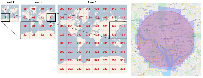
Now let’s consider tree-based approaches - there are four we will go over: Quadtree, R-Tree, Google-S2, and Uber-H3.
Quadtrees
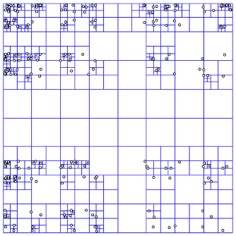
The Quadtree recursively divides the map based on a specified criteria such as the number of points of interest in the cell rather than the cell area. Each subdivided cell is further subdivided until each cell contains less than X points of interest. The Quadtree is an in-memory only data structure unlike Geohashing. Each internal node is represented by 4 numbers (2 pairs of coordinates: NW and SE corners) and pointers to 4 children, which is roughly 64 bytes ((8 bytes * 4) + (8 bytes * 4)). With 500 million points of interest, if we allow up to 100 points per leaf node, that is 5 million leaf nodes. Each leaf node is represented by 4 numbers (2 pairs of coordinates) and up to 100 point of interest IDs which is roughly 832 bytes ((8 bytes * 4) + (8 bytes * 100)). Internal nodes in a Quadtree are typically ⅓ the number of leaf nodes, which gives us another 1.67 million internal nodes, for a total of 6.67 million nodes. The total in-memory space requirements therefore is 4.21GB ((5 million * 832) + (1.67 million * 32)).
Quadtrees provide more even groupings of points of interest, individual subtrees can be incrementally rebuilt when new points of interest are added/removed, support k-nearest points queries, and dynamically adjust cell size based on density. Since the quadtree is in-memory it needs to be rebuilt if the server it is stored on is restarted. Quadtrees are a bit more complex to implement, such as rebalancing when adding/removing points from a quad tree. Quadtrees are also commonly used in image representation, processing, and compression.
R-Trees
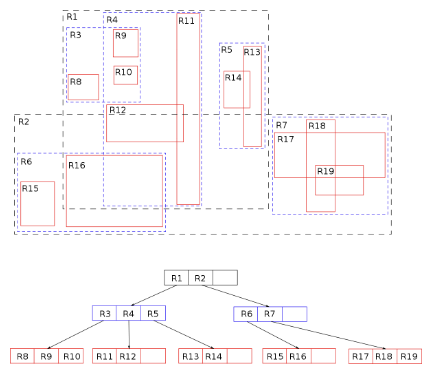
R-Trees are similar to Quadtrees - the R-Tree is also a tree data structure with the root representing the largest geospatial area and child nodes representing sub-areas of the parent. Unlike Quadtrees, R-Trees child node spatial areas may overlap and the tree remains balanced as nodes are added/removed. R-Trees are generally faster than Quadtrees at k-nearest-neighbors queries. Constructing a R-Tree is generally quicker than constructing a Quadtree too as it requires less space. For data that is rapidly changing, Quadtrees generally perform better. Finally, R-Trees can be extended to more than just 2 dimensions for other use-cases. A neat simulation comparing Quadtree and R-Tree can be viewed here.
Google S2
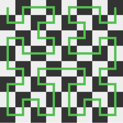
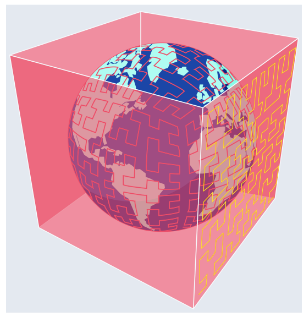
Google’s S2 takes a different approach by modeling a 3D globe and projecting points from the 3D sphere onto a 3D cube encompassing the globe. As points are projected onto the 3D cube, each 2D cube-face is transformed into 1D space as a Quadtree using the Hilbert Curve. The first bits identify the cube face, while the remaining bits identify the position on the Hilbert Curve. The Hilbert Curve is a space-filling curve where every latitude+longitude point in 2D space is located as a single point on the Hilbert Curve while maintaining spatial locality between points. The Hilbert Curve is especially useful because it has an important property: two points close in 2D space are guaranteed to be close to each other on the Hilbert Curve in 1D space. S2 supports 30 levels of resolution and is well suited for geofencing applications with its region cover algorithm mixing different-sized cells for optimal efficiency.
Uber H3
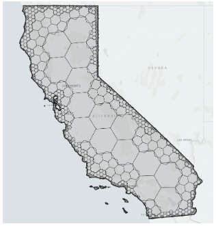
Lastly, we have Uber’s H3 approach. Uber’s H3 and Google’s S2 both use 64-bit integers as cell indexes with the main difference between the two being the shape of their cells. Uber H3 uses hexagons to represent spatial areas rather than squares which results in centroids which are equidistant. Google S2 with square cells is preferable for use cases where exact aggregation and subdivision are needed, whereas Uber H3 with hexagonal cells is preferable for use cases where neighbors and grid traversal are important.
As you can see Geohashing and the various tree-based approaches work well, though with different trade-offs to consider for various use-cases. This covered these approaches at a high-level and I recommend digging deeper into whichever approaches best fit your use-case before you begin system design and implementation.